Lab 03
Conditional Formatting Practice
Three lab files from the MOS Excel Expert practice set. Work through Lab A and Lab C — they cover everything from this topic. Lab B is a bonus for fast finishers.
How to check your work
Each lab has a results file — open it side by side with your work and compare visually. You can also open Home → Conditional Formatting → Manage Rules in the results file to inspect exactly how each rule was built. Screenshots on this page show the visual outcome only — the rules are in the results file.
Lab Order
Lab A · Everyone
ExcelExpert_2-3a — Visual & Predefined Rules
Three worksheets, three different visual formatting techniques. No formulas required — these use the built-in rule types from the Conditional Formatting menu.
Download ExcelExpert_2-3a.xlsx1
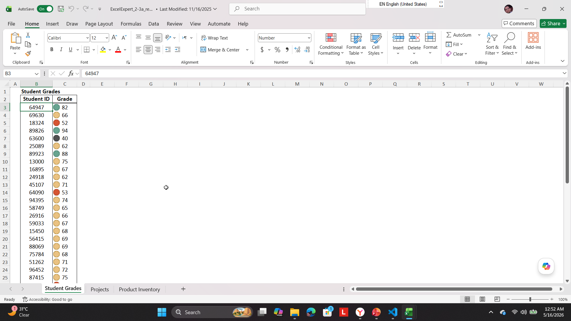
Student Grades worksheet — Traffic Light Icon Set
Apply a 4 Traffic Lights icon set to the Grade column using custom value thresholds:
- ⚫ Black icon — values less than 50
- 🔴 Red icon — values 50 to 59
- 🟡 Yellow icon — values 60 to 79
- 🟢 Green icon — values 80 and above
2
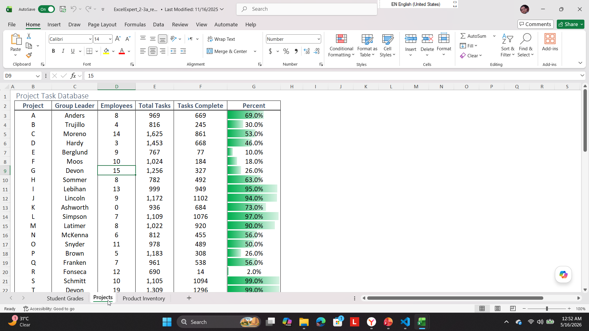
Projects worksheet — Data Bar with custom range
Apply a green gradient Data Bar to the Percent column. Set a custom minimum of
0 and maximum of 1 — the values are stored as decimals so the bar must be calibrated to that scale.
3
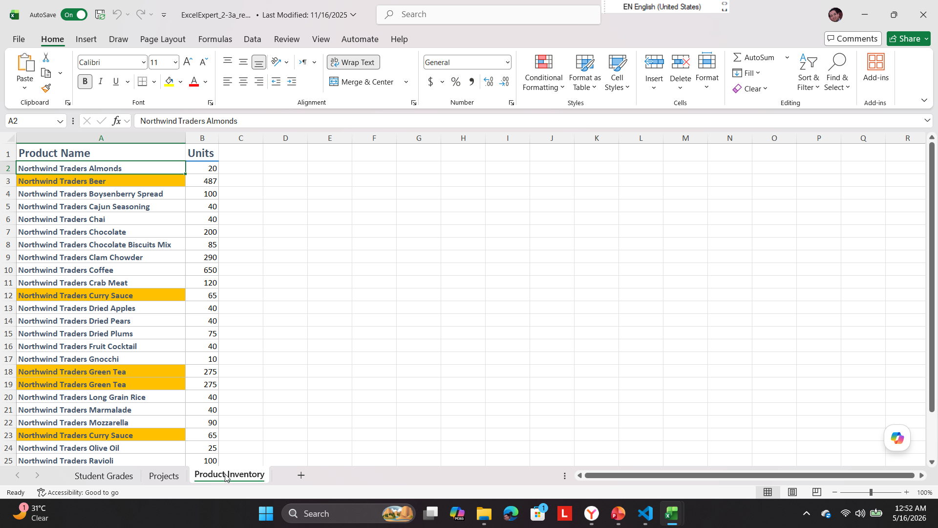
Product Inventory worksheet — Duplicate values
Apply an orange fill to any duplicate product names in the Product Name column.
Lab C · Everyone
ExcelExpert_2-3c — Managing & Editing Rules
Two overlapping rules on the same range — then edit one and reorder them. This is where most people discover that rule order matters.
Download ExcelExpert_2-3c.xlsx1
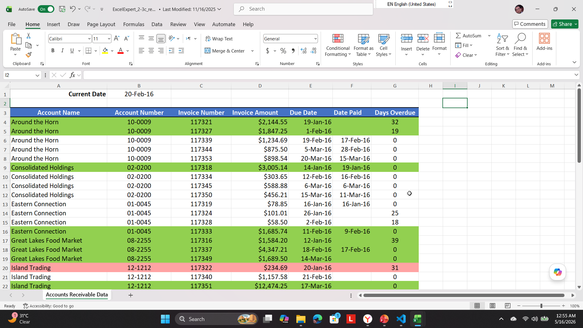
Accounts Receivable worksheet — Two rules, one range, then edit & reorder
Work on range
A4:G55. Apply these two formula rules in order:
- Light green fill — rows where Invoice Amount > $2,000
- Orange fill — rows where Days Overdue ≥ 30
- Edit the first rule — change the threshold from $2,000 to $1,500
- Open Manage Rules and move the Invoice Amount rule above the Days Overdue rule
- Observe how the result changes when a row qualifies for both rules
Rule order in Manage Rules
When two rules apply to the same cell, the one higher in the list wins — unless "Stop If True" is checked. Reordering rules is how you control which format takes priority when conditions overlap.
Lab B · Bonus — Fast Finishers
ExcelExpert_2-3b — Formula-Based Rules
Three formula-driven tasks. These extend the Advanced techniques from Topic 03 — same approach, new scenarios and functions.
Download ExcelExpert_2-3b.xlsx1
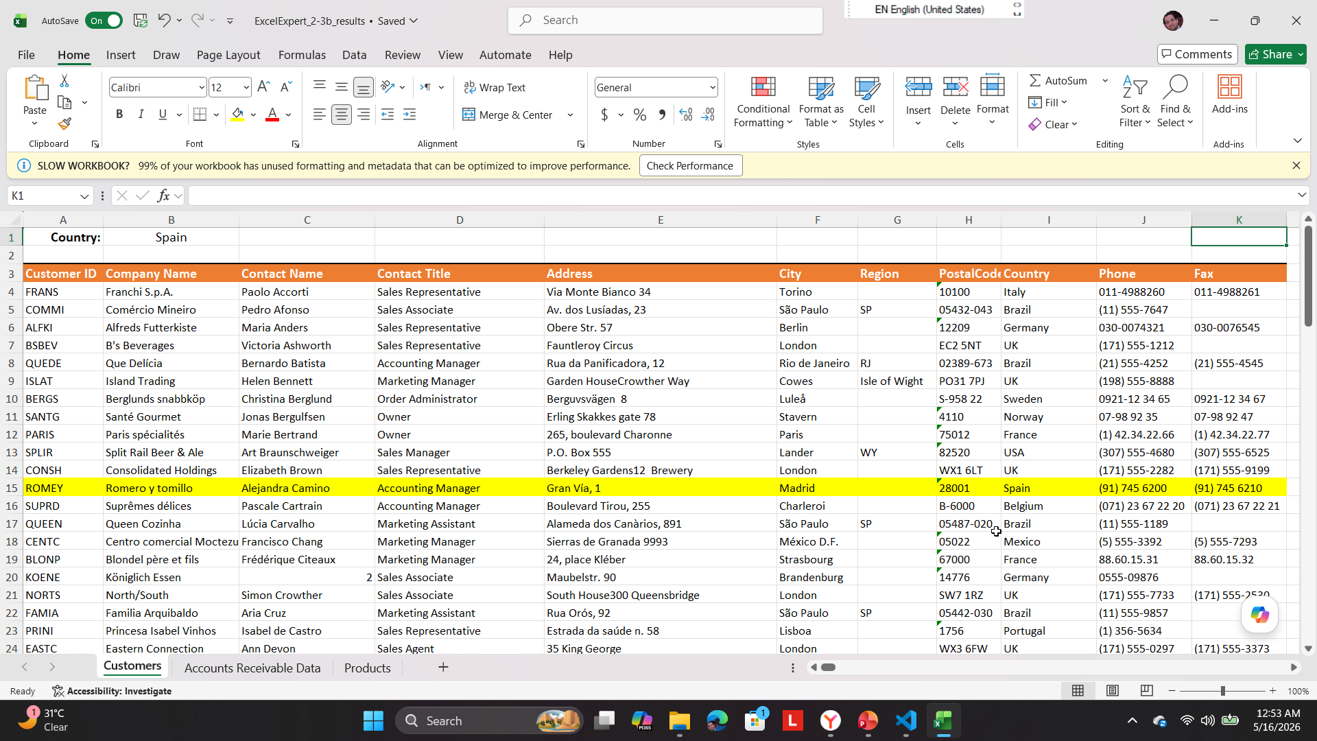
Customers worksheet — Highlight rows matching a reference cell
Range
A4:K94. Write a formula rule that applies a yellow fill to the entire row when the country in column I matches the value typed in cell B1.
- After applying, change the country in
B1— the highlighted rows should update instantly
Hint: Think about which references need locking. The country column (I) should stay fixed — the row should move freely. Cell B1 is a fixed lookup point and needs both row and column locked.
2
Accounts Receivable worksheet — Stripe every other row using MOD
Range
A4:G55. Use MOD and ROW() to apply a light grey fill to every other row.
- After applying, delete a row — the striping should re-adjust automatically without any manual update
Hint:
MOD(ROW(), 2) returns 0 for even-numbered rows and 1 for odd-numbered rows. Look up MOD in Excel Help if needed — finding and reading function documentation is part of this task.
No screenshot for this task — the key test is deleting a row and confirming the striping re-adjusts automatically.
3
Products worksheet — Highlight the highest and lowest rows
Range
A2:B78. Apply a red fill and bold font to the entire rows that contain the highest and lowest values in the Change In Units Sold column.
- After applying, type a new high or low value — the formatting should shift to the new winner automatically
Hint: This is a variation of Advanced 02 from Topic 03 — but the format applies to the whole row, not just a single cell. Think about how the column reference changes when you want the rule to cover both columns A and B.