Topic 14
Advanced Pivot Tables
Take your pivoting skills further. Learn how to present multiple Pivot Tables side-by-side on a single worksheet, link them to a single slicer across the entire workbook, and group numeric values (like salaries) into defined bracket ranges.
Step 1 — Side-by-Side Pivot Tables
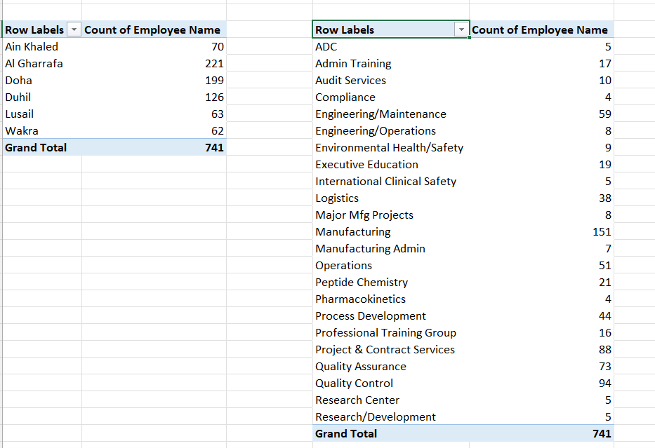
You are not limited to one Pivot Table per sheet. Placing tables side-by-side allows users to compare different dimensions of the same dataset (such as Building headcount vs. Department headcount) at a glance.
E1).The two summaries will render side-by-side on the same sheet (pivot8):
Step 2 — Slicers and Report Connections
Slicers are visual filters. When you add a Slicer, it is initially linked only to the Pivot Table that was active when it was created.
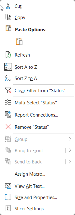
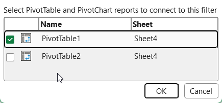
To control both Pivot Tables with the same slicer, we use **Report Connections** (pivot10):
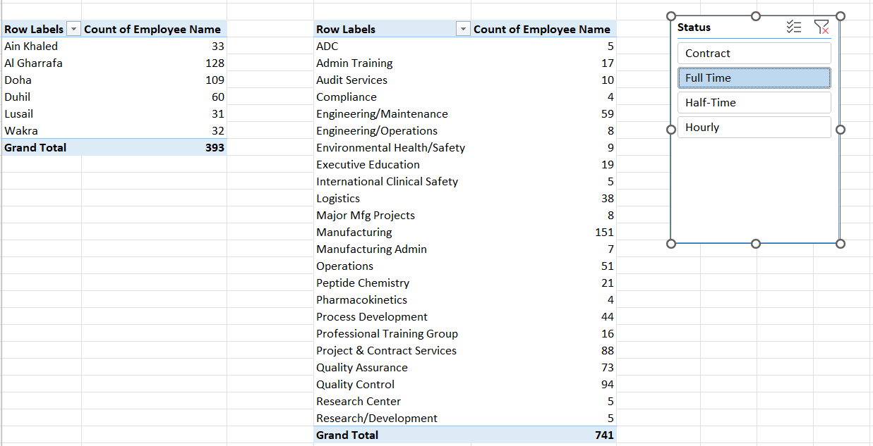
Once report connections are enabled, selecting "Full-time" on the slicer correctly filters both tables simultaneously (pivot11):
Step 3 — Grouping Numerical Data into Brackets
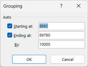
What if you need to classify staff into salary ranges? (e.g. how many make $1–$10,000, how many $10,001–$20,000, etc.)? Excel allows you to group numerical row labels into even bracket intervals instantly.
• Starting at:
1 (By default, Excel inputs the smallest cell value, but you can override it).
• Ending at:
90000 (or keep it checked for auto-max).
• By:
10000 (the size of each bracket). Click OK.
Self-Check — Verify Your Advanced Pivot Output
Build the side-by-side pivot tables and grouped salary table inside StaffData.xlsx, then check your figures below.
| Summary Metric | Your Value |
|---|---|
| Headcount in Logistics Department | |
| Headcount in Manufacturing Department | |
| Staff with salaries in the $1–$10,000 range | |
| Staff with salaries in the $40,001–$50,000 range |