Lab · Lookup Functions
Lookup Practice
Three tasks in one workbook — each targeting a different lookup technique. Tasks 1 and 2 use approximate match. Task 3 is a two-dimensional lookup where both the row and the column are dynamic.
How to check your work
Download the results file and open it side by side with your work. For Tasks 1 and 2, click "Show Result" to see the expected output on this page. For Task 3, compare your formula logic against the breakdown below — then verify with the results file.
MOS Excel Expert — Objective 3.2
ExcelExpert_3-2 — Lookup Functions
Three worksheets, three techniques. Work through them in order — each one builds on the previous topic.
Download ExcelExpert_3-2.xlsx Lab Instructions (PDF)1
Tax Rate worksheet — VLOOKUP approximate
Add a formula to cell B18 that looks up the income in B17 against the tax table in C9:F15 and returns the applicable tax rate.
Refer to: Topic 06 — VLOOKUP Approximate
Hint
This is the same bracket-lookup pattern from Topic 06. The income in B17 falls within a range — use VLOOKUP with
1 as the 4th argument. Count which column in C9:F15 holds the tax rate to determine the column index number. Lock the table range with $.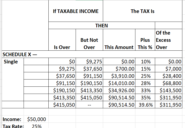
2
Discount Schedule worksheet — HLOOKUP approximate
Create formulas in D3:D10 that look up the units ordered in A3:A10 against the discount schedule in B13:G14 and return the applicable discount percentage.
New: HLOOKUP — see explanation below
Function introduced in this lab
HLOOKUP — horizontal VLOOKUP
HLOOKUP is VLOOKUP rotated 90°. Instead of searching down a column and returning from a column to the right, it searches across a row and returns from a row below. Same 4 arguments, same 3 problems — including approximate match by default.
= HLOOKUP(lookup_value, table_array, row_index_num, [range_lookup])
VLOOKUP
Searches down column 1
Returns from a column to the right
3rd arg = column number
Returns from a column to the right
3rd arg = column number
HLOOKUP
Searches across row 1
Returns from a row below
3rd arg = row number
Returns from a row below
3rd arg = row number
The discount table
B13:G14 has unit quantities in row 1 and discount percentages in row 2. Use 2 as the row index number. The units fall in brackets → approximate match → use 1 as the 4th argument. Lock the table with $ so it stays fixed as you copy the formula down.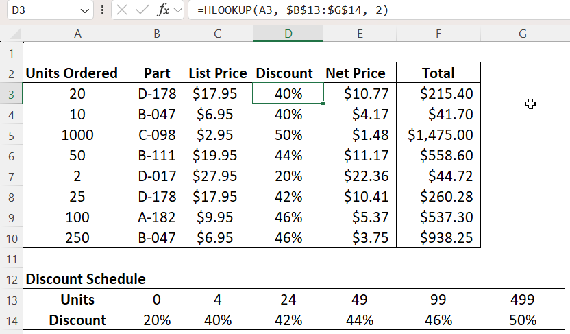
3
Parts worksheet — INDEX + MATCH + MATCH (2D dynamic lookup)
Add a formula to cell B3 that uses the range A7:H14 to look up the part number in B1 and return the value from the field whose name is in B2.
Refer to: Topic 08 — MATCH & INDEX
Reading the task
B1 = Part Number (e.g. "D-017") — this is the known value to search for.
B2 = Field Name (e.g. "Cost") — this decides which column to return from.
B3 = the formula result. Changing either B1 or B2 should update the result automatically.
B2 = Field Name (e.g. "Cost") — this decides which column to return from.
B3 = the formula result. Changing either B1 or B2 should update the result automatically.
Formula Breakdown — Build it in three layers
MATCH(B1, H8:H14, 0)
Find which row — search for the part number (B1) in the Number column (H8:H14). The part numbers are in the last column of the data. Returns the row position.
MATCH(B2, A7:H7, 0)
Find which column — search for the field name (B2) in the header row (A7:H7). Returns the column position. This is what makes the lookup dynamic — change B2 and a different column is returned.
INDEX(A8:H14,
MATCH(B1,H8:H14,0),
MATCH(B2,A7:H7,0))
MATCH(B1,H8:H14,0),
MATCH(B2,A7:H7,0))
Combined formula — INDEX returns the value from the data grid (A8:H14) at the intersection of the row found by the first MATCH and the column found by the second MATCH. This is the complete answer for B3.
Test your formula
With B1 = "D-017" and B2 = "Cost", the result should be $18.69. Change B2 to "Description" — the result should change to Langstrom 7" Wrench. Both the row and the column are fully dynamic.
No screenshot for this task — verify with the results file and the test values above.